
DFF Sensor: Inline Rheometery. Shear Rate
November 8, 2021 2023-11-14 21:48DFF Sensor: Inline Rheometery. Shear Rate
DFF sensor: Inline Rheometry in Powder and Liquid Flows. Shear Stress and Shear Rate Measurement.
Drag force flow (DFF) measurement is a technique for continuous inline characterization of powders, slurries, or liquids during processing. Like conventional off-line rheometry, such as dynamic testing, it is based on measurement of forces associated with the movement of powders or liquids.

Flow force measurement technology
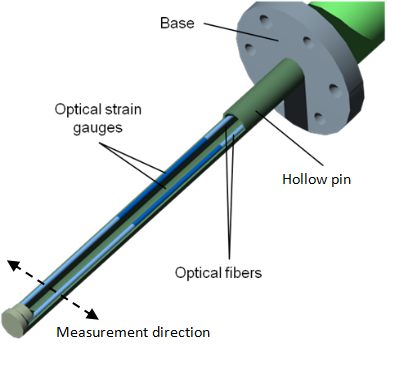
Lenterra’s inline measurement tool, a drag force flow (DFF) sensor, is a needle-like probe. Flow around the pin causes its deflection, the magnitude of which is measured with high sensitivity by a pair of optical strain gauges or Fiber Bragg Gratings (FBGs) mounted within its hollow core.
The extent of deflection is directly related to the force exerted on the pin. This force is a function of the properties of the in-process material flow including the velocity of movement, particle/fluid density and/or viscosity. The Evolution of the measured force as a function of time can therefore be correlated directly with process behavior and critical process parameters. In addition to force, the optical assembly of the DFF sensor measures the temperature of the flow material. Information is collected via optical fibers that connect the FBGs within the sensor to an optical interrogator.
DFF sensor can be installed into a vessel or line for continuous powder or liquid flow measurement. Miniature design and optical measurement principle of the sensor give it several important advantages for in-process monitoring. For example, measurements are unaffected by electromagnetic interference or the build-up of material at the sensor surface (fouling), the sensor self-calibrates for temperature and there is no ignition hazard. A measurement rate of 500 cycles per second provides essentially continuous monitoring enabling the generation of highly repeatable data and the characterization of any periodicity associated with processes such as mixing, blending and granulation.
See more detail of the DFF sensor measurement technology in our White Paper 1.
Process characterization metrics: force pulse magnitude (FPM), pulse consistency factor (PCF) and amplitude at process frequency (APF)
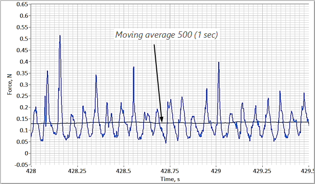
The figure presents a 1.5-second-long measurement of flow force detected by a DFF sensor inserted into the wet mass during granulation of a placebo formulation in a 10-liter GEA PharmaConnect® granulator. The plot features periodic pulses corresponding to the events of agitator blades periodically passing by the sensor probe. Such an evolution provides information about an averaged in time flow force (shown with the moving average line) as well as about mass and density of individual granules which are responsible for magnitudes of peaks on the plot. Having information about multiple blade actions in a short period of time calls for application of standard statistical methods. The three basic metrics that are deduced from the “raw” measurement are force pulse magnitude (FPM) pulse consistency factor (PCF), as well as amplitude at process frequency (APF).
Mean force pulse magnitude (MFPM) and pulse consistency factor (PCF)
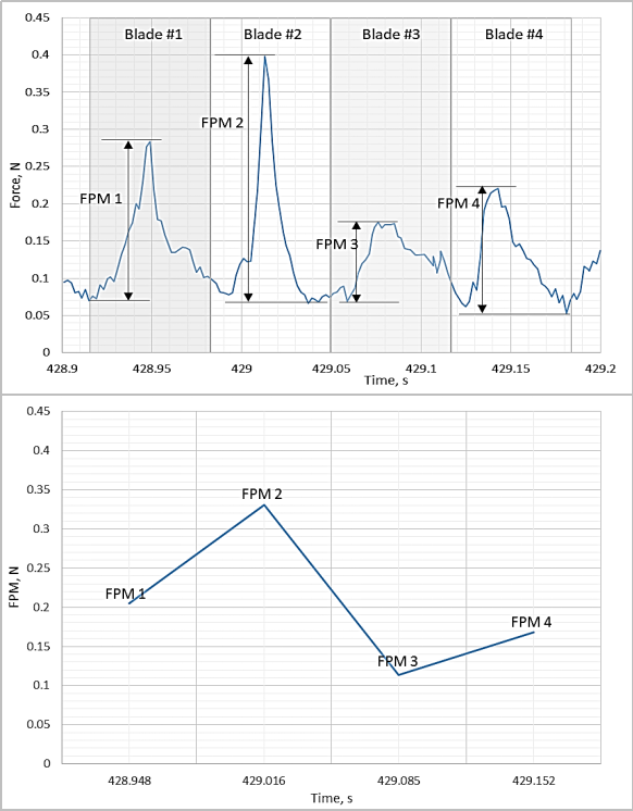
Values of FPM are obtained by plotting the difference between the highest and lowest values of force measured in a specific time period (see figure). The time period associated with this calculation is the process frequency, which is the frequency of rotation of the agitator multiplied by the number of blades. FPM values are always positive and provide a useful metric for the evaluation of flow characteristics, though useful information can be extracted from an analysis of individual force pulses as well.
FPM values can be displayed as a rolling average, a common approach in process control. It is also possible to derive further metrics for process characterization by considering arrays of consecutive FPM values. An array contains a certain number of FPM values that can be processed statistically to produce an “instantaneous” histogram.
The exemplary probability histogram for an array of FPM values is shown in the figure was generated from 300 FPM data points gathered over a 20-second timeframe. A log-normal distribution fit applied to such histograms generates two independent parameters: the mean value, MFPM, and the width of the distribution, WFPM. By advancing in very small increments of time to generate successive, overlapping histograms, as with a moving average, changes in MFPM and WFPM can be determined to monitor the evolution of a process.
In terms of practical significance, MFPM reflects average particle size and density while WFPM is a measure of diversity in the process material, and may be indicative of, for example, the uniformity or cohesiveness in the powder. These two metrics can be further used to determine a parameter called the Powder Consistency Factor, PCF = MFPM/WFPM, which characterizes the uniformity of the flow force. For example, in a system consisting predominantly of fine particles but containing a number of large agglomerates intermittently interacting with the probe, WFPM will be high resulting in a low PCF. The benefit of using PCF in place of WFPM is that it is a unitless parameter, normalized with MFPM, essentially with particle mass-size.

Process fingerprint
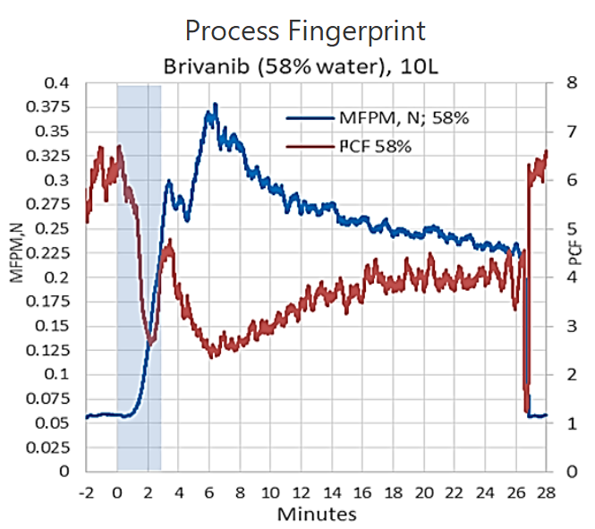
Evolutions of MFPM and PCF over the length of the process constitute process signatures. Together, MFPM and PCF provide a fingerprint for the process. An example of such a fingerprint for processing Brivanib Alaninate in a 10L GEA PharmaConnect® granulator is presented in the figure. It shows several salient features in both MFPM and PCF evolutions that are indicative of granulation stages. Two characteristic maxima on the FPM signature and the corresponding to them minima in the PCF signature may be used for granulation end point determination and/or scaling.
More information about FPM and PCF metrics is found in our White Papers 3 and 13.
FPM and PCF signatures can be used for any processing that involves periodic change in flow velocity. Applications range from powder processing in mixers, granulators, dryers, etc. through processing of slurries to processing of liquids such as protein mixing and pump action analysis. The approach also provides a sensitive characterization of raw materials (White Paper 16).
Fluid Uniformity
Uniform homogeneous fluid will generate the same values of shear stress from one blade to another which manifest themselves as pulses of the force on the force vs. time evolution. Principal metrics of LIR technology are force pulse magnitude (FPM) and pulse consistency factor (PCF), see detailed description in our White Papers 3 and 13 . Any fluctuation in the fluid density and/or viscosity will result in fluctuation of FPM from one blade to another. Recording several (typically more than 50) FPMs in sequence, one may construct a histogram or distribution of the FPM values. The width of such a distribution would characterize the uniformity of the flow material. A narrow distribution of FPMs indicate high homogeneity and a wider one – a less uniform fluid. This analysis is provided by the LENFLOW measurement software in real time and reported as PCF (pulse consistency factor). The higher PCF value the more homogeneous fluid material is.
Amplitude at process frequency (APF)
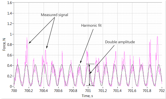
APF is another metric obtainable from the periodic signal of flow force in mixers. It is the amplitude of the harmonic fit to the raw data.
The total signal in this approach is modeled with
F(t)=F_0+A_0\ sin(2πft+φ)
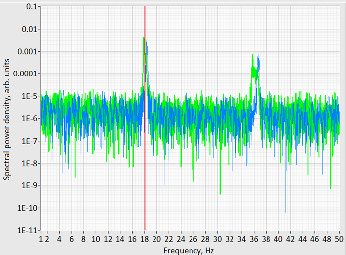
Here is the continuous, steady component of the force, is APF, is the process frequency and is the initial phase. The process frequency is the frequency of the blades passing near the probe. It is the RPM multiplied by the number of blades in the agitator. The process frequency can be known prior to the measurement or obtained from raw force data by applying fast Fourier transformation (FFT) as demonstrated in the FFT spectrum in the figure.
APF averages magnitudes of all peaks therefore the doubled APF can be understood as an average difference between the maximum and minimum force exerted on the probe. APF is therefore is the amplitude of alternating component of the force, whereas is the steady component.
APF is specifically useful for measuring shear rate in liquids since it represents the force exerted by the one part of the flow to another.
Calculating velocity or viscosity in liquids
Connection between the force on the probe and velocity can be understood as follows.
The drag force exerted by uniform flow on a cylinder is:
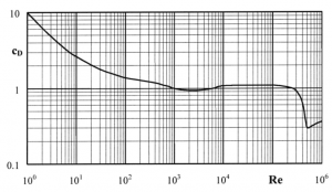
F=C_d Aρu^2/2
where Cd is a drag coefficient for the cylinder, A=2r_0 l is the cross section of the pin, ρ is the fluid density, u is flow velocity, l is the length of the pin, r_0 is the outer radius of the pin. C_d is a function of the Reynolds number, Re=(2r_0 uρ)/μ , where μ is the fluid viscosity. The dependence of drag coefficient on Reynolds number is well known and can be graphically represented as shown in figure. Solving these two equations numerically allows for calculating flow velocity at the probe location provided the viscosity of the fluid is known.
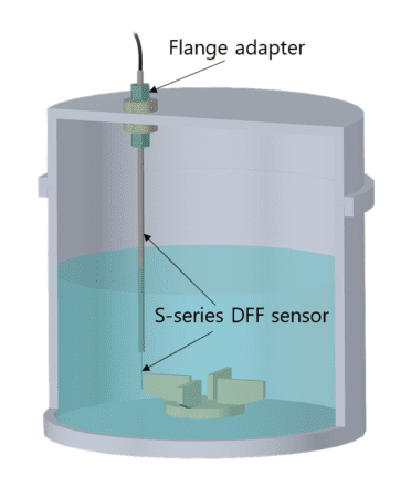
If velocity is known, drag coefficient C_d is calculated as C_d=2F/Aρu^2. Knowing dependence C_d(Re) the Reynolds number is numerically found and then dynamic viscosity is computed as μ=2r_0uρ/Re. In mixers, when the DFF sensor is positioned close to the edge of the agitator blade as in the figure below, the flow velocity could be approximated with the velocity of the agitator blade edge.
Shear stress
DFF sensor probe positioned vertically in a mixer measures, depending on its measurement axis direction, either tangential or radial component of the shear force exerted on the probe by the fluid. This force F, a direct output of the LENFLOW measurement software, is related to the shear stress experienced by the surface of the pin as
τ=C F/A_s
Here τ is the shear stress, A_s=2πr_0 l is the surface area of the pin, l is the length of the pin, and r_0 is the outer radius of the pin, C is a geometric coefficient that depends on the portion of the pin submerged into the fluid. Since DFF sensor measures a component of the force that is parallel to its measurement direction, the measured stress is also a component in same direction. The second component can be measured by rotating the cylindrical probe 90 degrees around its axis.
Shear rate calculation
The shear rate is the rate of change in velocity at which one layer of fluid passes over an adjacent layer. Knowing difference in velocities Δu at two points along a certain direction and the distance between these points, Δr, the shear rate is
\dot{γ} = Δu/Δr
Depending on the direction of the flow there could be several components of shear rate, which can be measured separately. In a cylindrical mixer, LIR-D can measure the tangential component due to tangential velocity \dot{γ}_{t,t}, tangential component due to radial velocity \dot{γ}_{r,t}, radial component due to tangential velocity \dot{γ}_{t,r}, and radial component due to radial velocity \dot{γ}_{r,r}.
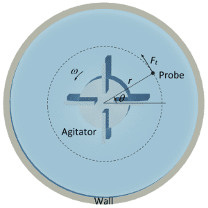
Tangential component of shear rate due to tangential velocity
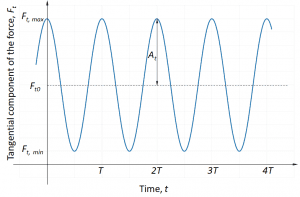
Assuming that the sensor position vertically and its measurement direction is tangential as shown on the schematics, the measured force represents a tangential component of the total force exerted on the pin. This force will be changing periodically in time, in a simple case sinusoidally. For one full turn of the agitator, there will be four (in this example) full periods of force change, T=1/f =1/4 (2π/ω) , where f is the process frequency and ω is the angular frequency. Therefore, since the sensor measures the tangential component, and the force evolution can be approximated as
F_t (t)=F_{t0}+A_t \ sin(4ωt+φ)
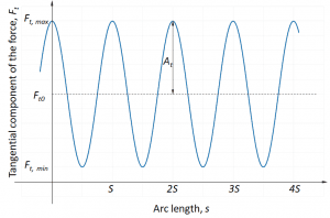
Where F_{t0} is the is the continuous, steady tangential component of the force. Since the flow does not change its properties significantly over one rotation of the agitator, after measuring the force over one rotation of agitator, one obtains tangential force component distribution over the circumference of the circle of radius r .
F_t (s)=F_{t0}+A_t\ sin (Nθ+φ)= F_{t0}+A_t\ sin(N s/r+φ)
Here angle θ changes between zero and 2π, and arc length s=θr varies between zero and 2πr. N is the number of blades in the agitator that is 4 in our example. S is the length of the period on the F_t (s) plot. One can see that the change in force between the maximum and minimum of the sinusoidal fit occurs over a half-length of the period S/2. From the maximal and minimal forces, F_{t,max}= F_{t0}+A_t and F_{t,min}= F_{t0}-A_t, respectively, we can calculate the maximal, u_{t,max} and minimal, u_{t,min} velocity of the fluid at the circumference of radius r. The difference between these velocities divided by the distance between them is the tangential component of the shear rate for tangential component of flow velocity:
\dot{γ}_{t,t} = Δu_t/Δr_t ≅2N(u_{t,max}-u_{t,min})/2πr
Force amplitude A_t is found by applying the APF algorithm.
Tangential component of shear rate due to radial velocity
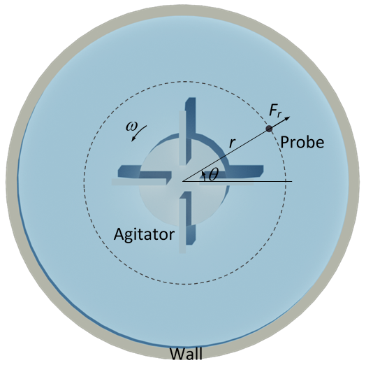
If the sensor is rotated so that it sensitivity axis is aligned with the radial direction in the mixer, the measured force is due to fluid motion in radial direction. Similarly to the measurement for tangential velocity, radial force distribution over the circumference of the circle is measured over one complete turn of the agitator and given by
F_r (s)=F_r0+A_r sin (Nθ+φ)= F_r0+A_r sin(N s/r+φ)
Using the same approach as that for calculation of tangential-tangential component of the shear rate, calculation of tangential-radial component involves finding velocities u_{r,max} and u_{r,min} from the minimal and maximal forces over one period, and dividing them by the distance between them along the circumference of radius r: \dot{γ}_{r,t}=(Δu_r)/(Δr_t )≅(u_{r,max}-u_{r,min})/2πr 2N
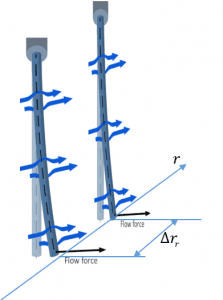
Radial components of shear rate due to tangential and radial velocities
Determining radial component of shear rate requires force measurements in two different radial positions within the mixer. This can be done using two DFF probes spaced by a few millimeters.
Alternatively, a single sensor can be used. The velocity difference is found by taking a first measurement, then moving the sensor along the radius for a distance of Δr and taking the second measurement. For calculating the radial component of shear rate due to tangential velocity, \dot{γ}_{t,r}=Δu_t/Δr_r, the sensor measurement axis should be perpendicular to radius, and for finding the radial component due to radial velocity, \dot{γ}_{r,r}=Δu_r/Δr_r , the sensor measurement axis should be aligned with the radius.